ICU Mortality: Interpretable Inference Meets Predictive Power

Biostatistics

Machine Learning

Clinical Risk Modeling

Two models on 91,713 ICU admissions: an interpretable logistic regression for clinical inference, and a cross-validated LightGBM (AUC 0.90) for prediction, with an honest accounting of why the two AUCs differ.

Published

May 4, 2026

The question

Which patient characteristics and first-day ICU measurements are most associated with in-hospital mortality, and how much predictive performance do you trade away by insisting on a model clinicians can actually read?

I answered both halves with a deliberate two-track design: an interpretable logistic regression for inference, and a gradient-boosted LightGBM for predictive performance, compared honestly on the same cohort.

Data

The WiDS Datathon 2020 (GOSSIS) cohort: 91,713 ICU admissions across 186 variables, spanning demographics, admission context, comorbidity flags, and first-day vitals and labs. Overall mortality was about 9%, a meaningful class imbalance the models had to handle.

The two tracks used the data differently, on purpose.

Logistic track. A parsimonious 10 predictors, complete-case (71,926 rows), every coefficient interpretable. Lactate (about 75% missing) was dropped rather than imputed on weak ground, and I ran a complete-case selection-bias check. Retained versus dropped patients had near-identical mortality (8.5% versus 9.0%), which is what makes complete-case analysis defensible here rather than convenient.
LightGBM track. 72 features including APACHE components and comorbidity flags, with no row-dropping, since gradient boosting routes missing values through its splits natively.

Method

Logistic regression with pre-ICU length of stay log-transformed for skew. Multicollinearity was checked explicitly through a correlation heatmap (BUN and creatinine at r ≈ 0.69, as expected for two renal markers) and VIFs (all below 2.1). Effect sizes were rescaled by each predictor’s interquartile range, the figure below, so they read as “risk change across the middle 50% of patients” instead of uninformative per-unit odds ratios clustered near 1.0.

LightGBM tuned for binary classification with scale_pos_weight for the imbalance, evaluated by 5-fold stratified cross-validation, then refit on all data for a Kaggle submission pipeline (test-set categorical encoding aligned to training levels).

The IQR-scaled odds-ratio figure regenerates live from the fitted logistic coefficients, so it is fully reproducible without the raw 91k-row dataset.

library(dplyr)
library(ggplot2)
library(scales)

# Logistic-regression coefficients (log-odds scale) from the primary model on
# 71,926 complete-case admissions, with each continuous predictor's IQR.
# Reproduced from the model output for a self-contained figure.
coef_tbl <- tibble::tribble(
  ~label,               ~estimate,    ~se,        ~iqr,
  "Age",                 0.0175628,   0.0010024,  22,
  "Male gender",         0.0957692,   0.0290655,   1,
  "Elective surgery",   -1.1480364,   0.0525970,   1,
  "Pre-ICU LOS (log)",   0.2935830,   0.0217234,   0.3,
  "Min mean BP",        -0.0305368,   0.0010140,  20,
  "Min SpO2",           -0.0279573,   0.0010242,   6,
  "Max resp rate",       0.0165362,   0.0011609,   9,
  "Max creatinine",      0.0022678,   0.0107270,   0.7,
  "Max BUN",             0.0126412,   0.0007863,  18,
  "Max WBC",             0.0409460,   0.0016919,   7.3
) %>%
  mutate(
    or     = exp(estimate * iqr),
    lo     = exp((estimate - 1.96 * se) * iqr),
    hi     = exp((estimate + 1.96 * se) * iqr),
    effect = if_else(or < 1, "Protective", "Higher risk")
  )

p <- ggplot(coef_tbl, aes(x = or, y = reorder(label, or), color = effect)) +
  geom_vline(xintercept = 1, linetype = "dashed", color = "grey55") +
  geom_errorbarh(aes(xmin = lo, xmax = hi), height = 0.25, linewidth = 0.6) +
  geom_point(size = 3) +
  scale_x_log10(breaks = c(0.3, 0.5, 0.75, 1, 1.25, 1.5)) +
  scale_color_manual(values = c("Protective" = "#1F7A63",
                                "Higher risk" = "#15433C")) +
  labs(x = "Adjusted odds ratio per IQR (log scale)", y = NULL, color = NULL) +
  theme_minimal(base_size = 12) +
  theme(legend.position = "top", panel.grid.minor = element_blank())

Warning: `geom_errorbarh()` was deprecated in ggplot2 4.0.0.
ℹ Please use the `orientation` argument of `geom_errorbar()` instead.

`height` was translated to `width`.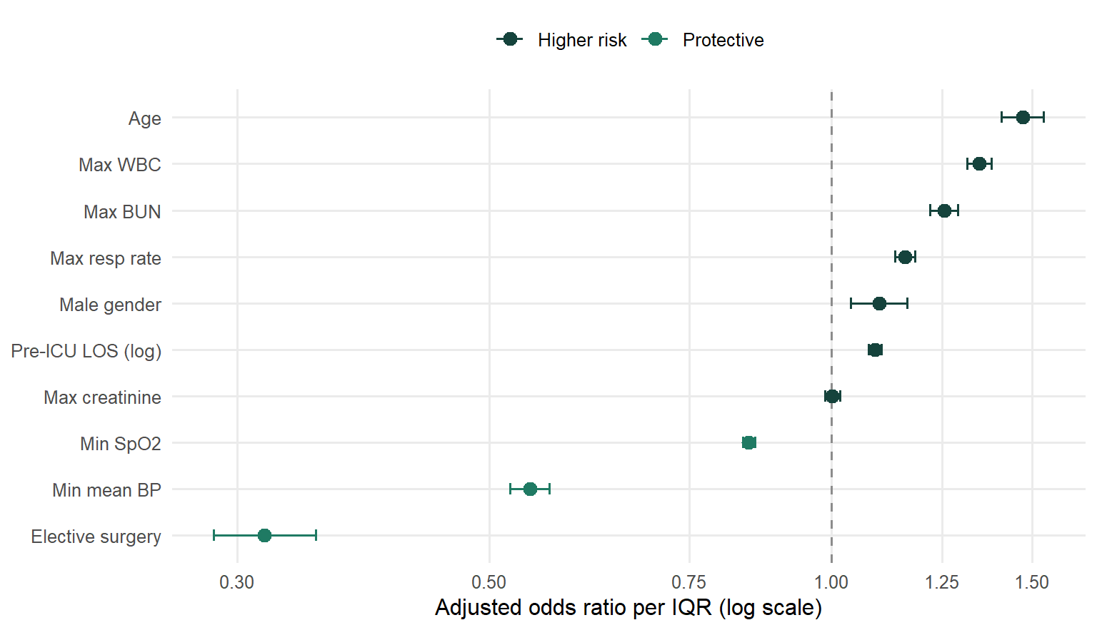

Figure 1: Adjusted odds ratios per interquartile-range increase. Points left of the dashed line are protective; points right are associated with higher mortality. Scaling by IQR makes clinical effect sizes directly comparable across predictors on different units.

Key results

Inference (logistic regression). Elective surgery was the strongest protective factor. Hemodynamic and respiratory instability (lower minimum mean BP, lower minimum SpO₂) and organ-stress markers (higher WBC, BUN, respiratory rate) raised risk, and age climbed monotonically across every decile. Creatinine was non-significant, and rather than wave it off, the VIF and correlation analysis show why: shared renal variance with BUN, not clinical irrelevance.

Prediction versus inference, reported honestly. This is the part worth dwelling on.

Two AUCs, reported honestly

Model	AUC	What kind of number this is
Logistic regression	0.784	Apparent (in-sample), optimistic
LightGBM	0.896	5-fold cross-validated, realistic

LightGBM’s cross-validated 0.896 (± 0.0035 across folds) genuinely beats the logistic model. But the logistic 0.784 is in-sample and therefore inflated, so the real performance gap is smaller than a naive 0.896-versus-0.784 reading suggests. Comparing a cross-validated number against an apparent one would be the kind of mistake that overstates a model, and flagging it is the point.

One caveat I would raise before a reviewer does: LightGBM’s top features are APACHE’s own pre-computed mortality probabilities (apache_4a_hospital_death_prob). So part of that 0.896 reflects the model successfully recovering an established clinical risk score already embedded in the data. That is legitimate, but worth naming rather than presenting the number bare.

Why it matters

This is the exact tension in applied clinical modeling. The interpretable model is what gets trusted, audited, and deployed at the bedside; the boosted model shows the ceiling of what is predictable. Doing both, and reporting the performance gap without inflating it, is the workflow real clinical-analytics and biostatistics teams use, and the methodological honesty is the transferable skill, more than either model alone.

Limitations

Stated plainly: the analysis is observational, so no causal claims. The logistic diagnostics (ROC, calibration, density separation) are apparent (in-sample); only the LightGBM AUC is cross-validated. Complete-case modeling drops about 22% of rows for the logistic track, which the bias check addresses but does not eliminate. And the 10-predictor logistic model trades discrimination for interpretability by design.

Links

📄 Read the full report covers the complete code, all exploratory figures, both models, CV results, and the Kaggle submission pipeline
💻 Code on GitHub
🗄️ Data: WiDS Datathon 2020 (GOSSIS)

adds <- c("/.quarto/", "/.Rproj.user/", "/_site/", "/_freeze/")
gi <- if (file.exists(".gitignore")) readLines(".gitignore") else character(0)
missing <- adds[!adds %in% gi]
if (length(missing)) cat("\n", paste(missing, collapse = "\n"), "\n", file = ".gitignore", append = TRUE)
writeLines(readLines(".gitignore"))   # print to confirm


 /.quarto/
/.Rproj.user/
/_site/
/_freeze/ 

 /.quarto/
/_freeze/ 

 /.quarto/
/_freeze/